Gibbs Sampling for Topic Models
Introduction
Suppose that we are under the situation that we want to discover the topics given a set of documents. What is the discovery of topics? It is to find out the values of the topic-related parameters in a topic model, such as pLSA or LDA. But, we cannot find the exact values of parameters of the model due to its complicatedness in calculating. So, we will estimate the parameters and this process is called inference in Bayesian approach. In this post, we will take the Gibbs sampling strategy for inference in LDA model.
Using Gibbs Sampling to Discover Topics
Generally, the estimation problem in LDA becomes one of maximizing the likelihood $p(\textbf{w}\vert \phi,\alpha)=\int p(\textbf{w}\vert \phi,\theta)p(\theta\vert \alpha)d\theta$, where $\textbf{w}$ represents the given documents and $p(\theta;\alpha)$ is a Dirichlet distribution with the parameter $\alpha$. But, the integral in this expression is known as being intractable in [1].
Instead of the above inference strategy, we will consider the posterior distribution over the topic assignments $p(z \vert \textbf{w})$ because what we are interested in is the distribution of topics given a document. Then, we will obtain estimates of $\theta$ and $\phi$ by examining this posterior distribution. And, we will take collapsed Gibbs sampling for inference problem. As for the collapsed Gibbs sampling, the general Gibbs sampling step for $z_i$, $p(z_i \vert \textbf{z}_ {-i}, \textbf{w}, \theta, \phi, \alpha, \beta)$, is replaced with a sample taken from the marginal distribution $p(z_i \vert \textbf{z}_ {-i}, \textbf{w}, \alpha, \beta)$, with the variables $\theta$ and $\phi$ integrated out, because this variation is tractable when $\alpha$ and $\beta$ are conjugate to $\theta$ and $\phi$ respectively.
The total probability of the model is
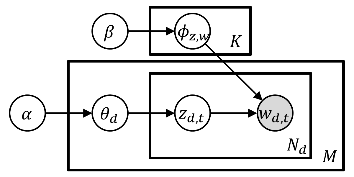
\[p(\textbf{w},\textbf{z},\mathbf{\theta}, \mathbf{\phi};\alpha,\beta)=\prod_{k=1}^K p(\phi_k;\beta)\prod_{d=1}^M p(\theta_d;\alpha)\prod_{t=1}^{c_d} p(z_{d,t}\vert \theta_d)p(w_{d,t}\vert \phi_{z_{d,t}})\]where $c_d$ denotes the length of document $d$.
Then, the joint distribution $p(\textbf{w},\textbf{z};\alpha, \beta)=p(\textbf{w}\vert \textbf{z},\beta)p(\textbf{z}\vert \alpha)$ by integrating out $\phi$ and $\theta$ is
\[\begin{aligned}p(\textbf{w}\vert \textbf{z},\beta)=&\int_{\phi}\prod_{k=1}^K p(\phi_k;\beta)\prod_{d=1}^M \prod_{t=1}^{c_d} p(w_{d,t}\vert \phi_{z_{d,t}})d\phi\\=&\prod_{k=1}^K \int_{\phi_k} p(\phi_k;\beta)\prod_{d=1}^M \prod_{t=1}^{c_d} p(w_{d,t}\vert \phi_{z_{d,t}})d\phi_k\\=&\prod_{k=1}^K \frac{\Gamma \left ( \sum_{v=1}^V \beta_v \right ) }{\prod_{v=1}^V \Gamma(\beta_v)}\frac{\prod_{v=1}^V \Gamma \left ( c_k^{(\cdot,v)} + \beta_v \right ) }{\Gamma \left ( \sum_{v=1}^V c_k^{(\cdot,v)} + \beta_v \right )}=\left ( \frac{\Gamma \left ( \sum_{v=1}^V \beta_v \right ) }{\prod_{v=1}^V \Gamma(\beta_v)} \right ) ^K \prod_{k=1}^K \frac{\prod_{v=1}^V \Gamma \left ( c_k^{(\cdot,v)} + \beta_v \right ) }{\Gamma \left ( \sum_{v=1}^V c_k^{(\cdot,v)} + \beta_v \right )}\\p(\textbf{z}\vert \alpha)=&\int_{\theta}\prod_{d=1}^M p(\theta_d;\alpha)\prod_{t=1}^{c_d} p(z_{d,t}\vert \theta_d)d\theta\\=&\prod_{d=1}^M \int_{\theta_d} p(\theta_d;\alpha)\prod_{t=1}^{c_d} p(z_{d,t}\vert \theta_d)d\theta_d\\=&\prod_{d=1}^M \frac{\Gamma \left ( \sum_{k=1}^K \alpha_k \right ) }{\prod_{k=1}^K \Gamma(\alpha_k)}\frac{\prod_{k=1}^K \Gamma \left ( c_k^{(d,\cdot)} + \alpha_k \right ) }{\Gamma \left ( \sum_{k=1}^K c_k^{(d,\cdot)} + \alpha_k \right ) }=\left ( \frac{\Gamma \left ( \sum_{k=1}^K \alpha_k \right ) }{\prod_{k=1}^K \Gamma(\alpha_k)} \right ) ^M \prod_{d=1}^M \frac{\prod_{k=1}^K \Gamma \left ( c_k^{(d,\cdot)} + \alpha_k \right ) }{\Gamma \left ( \sum_{k=1}^K c_k^{(d,\cdot)} + \alpha_k \right ) }\end{aligned}\]where $c_k^{(\cdot,v)}$ is the number of times that $v$th vocabulary has been assigned to topic $k$ in all documents, and $c_k^{(d,\cdot)}$ is the number of times that a word in document $d$ has been assigned to topic $k$.
The goal of Gibbs sampling here is to approximate the distribution:
\[p(\textbf{z}\vert \textbf{w},\alpha,\beta) =\frac{p(\textbf{z},\textbf{w}\vert \alpha,\beta)}{p(\textbf{w}\vert \alpha,\beta)}\]Since $p(\textbf{w}\vert \alpha,\beta)$ is invariable for any of $z$, the full-conditional distributions can be derived from the joint distribution $p(\textbf{z},\textbf{w}\vert \alpha,\beta)$ directly.
\[\begin{aligned}p(z_{(m,n)}=l\vert \textbf{z}_{-(m,n)}, \textbf{w},\alpha,\beta)=&\frac{p(z_{(m,n)}=l, \textbf{z}_{-(m,n)}, \textbf{w}\vert \alpha, \beta)}{p(\textbf{z}_{-(m,n)}, \textbf{w} \vert \alpha, \beta)}\\\propto&p(z_{(m,n)}=l, \textbf{z}_{-(m,n)}, \textbf{w}\vert \alpha, \beta)\\=&\left ( \frac{\Gamma \left ( \sum_{v=1}^V \beta_v \right ) }{\prod_{v=1}^V \Gamma(\beta_v)} \right ) ^K \prod_{k=1}^K \frac{\prod_{v \neq r} \Gamma \left ( c_k^{(\cdot,v)} + \beta_v \right ) }{1}\times \prod_{k=1}^K \frac{\Gamma \left ( c_k^{(\cdot,r)} + \beta_r \right ) }{\Gamma \left ( \sum_{v=1}^V c_k^{(\cdot,v)} + \beta_v \right )}\\&\times \left ( \frac{\Gamma \left ( \sum_{k=1}^K \alpha_k \right ) }{\prod_{k=1}^K \Gamma(\alpha_k)} \right ) ^M \prod_{d \neq m} \frac{\prod_{k=1}^K \Gamma \left ( c_k^{(d,\cdot)} + \alpha_k \right ) }{\Gamma \left ( \sum_{k=1}^K c_k^{(d,\cdot)} + \alpha_k \right ) }\times \frac{\prod_{k=1}^K \Gamma \left ( c_k^{(m,\cdot)} + \alpha_k \right ) }{\Gamma \left ( \sum_{k=1}^K c_k^{(m,\cdot)} + \alpha_k \right ) }\\\propto &\frac{\prod_{k=1}^K \Gamma \left ( c_k^{(m,\cdot)} + \alpha_k \right ) }{\Gamma \left ( \sum_{k=1}^K c_k^{(m,\cdot)} + \alpha_k \right )} \prod_{k=1}^K \frac{\Gamma \left ( c_k^{(\cdot,r)} + \beta_r \right ) }{\Gamma \left ( \sum_{v=1}^V c_k^{(\cdot,v)} + \beta_v \right )}\\=&\frac{\Gamma \left ( c_l^{(m,\cdot)} + \alpha_l \right )}{1} \cdot \frac{\prod_{k\neq l} \Gamma \left ( c_k^{(m,\cdot)} + \alpha_k \right ) }{\Gamma \left ( \sum_{k=1}^K c_k^{(m,\cdot)} + \alpha_k \right )}\\&\times \frac{\Gamma \left ( c_l^{(\cdot,r)} + \beta_r \right ) }{\Gamma \left ( \sum_{v=1}^V c_l^{(\cdot,v)} + \beta_v \right )} \prod_{k\neq l} \frac{\Gamma \left ( c_k^{(\cdot,r)} + \beta_r \right ) }{\Gamma \left ( \sum_{v=1}^V c_k^{(\cdot,v)} + \beta_v \right )}\end{aligned}\]where $z_{(m,n)}$ denotes the topic assignment of the $n$th word in document $m$, which corresponds to $r$th vocabulary, and $m \in { 1, \cdots, M }$ and $n \in { 1, \cdots, N_m }$.
Let $c_{k, -(m,n)}^{(d,t)}$ be the number of times that $t$th word in document $d$ has been assigned to topic $k$ excluding a topic which is assigned to the $n$th word in document $m$. The topic assigned to the $n$th word in document $m$ is $l$. So, $\Gamma \left ( c_l^{(m,\cdot)} + \alpha_l \right )$, for example, can be rewritten as $\Gamma \left ( c_{l,-(m,n)}^{(m,\cdot)} + \alpha_l + 1 \right )$.
\[\begin{aligned}p(z_{(m,n)}=l\vert \textbf{z}_{-(m,n)}, \textbf{w},\alpha,\beta)\propto&\frac{\Gamma \left ( c_{l,-(m,n)}^{(m,\cdot)} + \alpha_l + 1 \right )}{1} \cdot \frac{\prod_{k\neq l} \Gamma \left ( c_{k,-(m,n)}^{(m,\cdot)} + \alpha_k \right ) }{\Gamma \left ( \left ( \sum_{k=1}^K c_{k,-(m,n)}^{(m,\cdot)} + \alpha_k \right ) +1 \right )}\\&\times\frac{\Gamma \left ( c_{l,-(m,n)}^{(\cdot,r)} + \beta_r + 1\right ) }{\Gamma \left ( \left ( \sum_{v=1}^V c_{l,-(m,n)}^{(\cdot,v)} + \beta_v \right ) + 1\right )} \prod_{k\neq l} \frac{\Gamma \left ( c_{k,-(m,n)}^{(\cdot,r)} + \beta_r \right ) }{\Gamma \left ( \sum_{v=1}^V c_{k,-(m,n)}^{(\cdot,v)} + \beta_v \right )}\end{aligned}\]Then, the above equation is further simplified by treating terms not dependent on $l$ as constants, and we can conclude as follows using the property of Gamma function, $\Gamma(\alpha + 1)=\alpha \Gamma(\alpha)$:
\[\begin{aligned}p(z_{(m,n)}=l\vert \textbf{z}_{-(m,n)}, \textbf{w},\alpha,\beta)\propto&\frac{\Gamma \left ( c_{l,-(m,n)}^{(m,\cdot)} + \alpha_l + 1 \right )}{\Gamma \left ( \left ( \sum_{k=1}^K c_{k,-(m,n)}^{(m,\cdot)} + \alpha_k \right ) +1 \right )} \cdot \frac{\Gamma \left ( c_{l,-(m,n)}^{(\cdot,r)} + \beta_r + 1\right ) }{\Gamma \left ( \left ( \sum_{v=1}^V c_{l,-(m,n)}^{(\cdot,v)} + \beta_v \right ) + 1\right )}\\\propto&\frac{c_{l,-(m,n)}^{(m,\cdot)}+\alpha_l}{\sum_{k=1}^K c_{k,-(m,n)}^{(m,\cdot)} + \alpha_k} \cdot \frac{c_{l,-(m,n)}^{(\cdot,r)}+\beta_r}{\sum_{v=1}^V c_{l,-(m,n)}^{(\cdot,v)}+\beta_v}\end{aligned}\]Having obtained the full conditional distribution, the MCMC algorithm is then straightforward. The $z_{(m,n)}$ variables are initialized to values in ${1,2,\cdots,K}$, determining the initial state of the Markov chain. Then, the chain is run for a number of iterations, each time finding a new state by sampling each $z_i$ from the full conditional distribution. After enough iterations for the chain to approach the target distribution, the current values of the $z_i$ are recorded.
With a set of samples from the posterior distribution $p(\textbf{z}\vert \textbf{w})$, statistics can be computed by integrating across the full set of samples. For any single sample we can estimate $\phi$ and $\theta$ from the value $\textbf{z}$ by
\[\hat{\theta}_l^{(m,\cdot)}=\frac{c_l^{(m,\cdot)}+\alpha_l}{\sum_{k=1}^K c_k^{(m,\cdot)} + \alpha_k}\]
- The probability of topic $l$ in the document $m$
\[\hat{\phi}_l^{(\cdot,r)}=\frac{c_l^{(\cdot,r)}+\beta_{r}}{\sum_{v=1}^V c_l^{(\cdot,v)}+\beta_v}\]
- The probability of $n$th word $(=r)$ under topic $l$
Model Selection
The LDA model is conditioned on three parameters: the Dirichlet hyperparameters $\alpha$ and $\beta$ and the number of topics $K$. The above sampling algorithm is easily extended to allow $\alpha$, $\beta$, and $\textbf{z}$ to be sampled, but this extension can slow the convergence of the Markov chain. One strategy is to fix $\alpha$ and $\beta$ and explore the consequences of varying $K$. The choice of $\alpha$ and $\beta$ can have important implications for the results produced by the model. There are many ways for learning $\alpha$ and $\beta$, among which Minka’s fixed-point iteration is widely used. [3]
We update $\alpha$ and $\beta$ as follows:
\[\begin{aligned}\alpha_k^{\text{new}} \leftarrow& \alpha_k^{\text{old}} \cdot \frac{\sum_{m=1}^M \left [ \Psi \left ( c_k^{(d, \cdot)} + \alpha_k \right ) - \Psi (\alpha_k) \right ] }{\sum_{m=1}^M \left [ \Psi \left ( \sum_{k=1}^K c_k^{(d, \cdot)} + \alpha_k \right ) - \Psi (\sum_{k=1}^K \alpha_k) \right ] }\\\beta^{\text{new}} \leftarrow& \beta^{\text{old}} \cdot \frac{\sum_{k=1}^K \sum_{v=1}^V \left [ \Psi \left ( c_k^{(\cdot, v)} + \beta \right ) - \Psi (\beta) \right ] }{V \sum_{k=1}^K \left [ \Psi \left ( \sum_{v=1}^V c_k^{(\cdot,v)} + V\beta \right ) - \Psi (V\beta) \right ] }\end{aligned}\]In standard LDA model, a single scalar parameter $\beta$ is used as a hyperparameter on the exchangeable Dirichlet.
Collapsed Gibbs sampling
A collapsed Gibbs sampler integrates out one or more variables when sampling for some other variable. For example, suppose that a model consists of three variables $A$, $B$, and $C$. A simple Gibbs sampler would sample from $p(A\vert B,C)$, then $p(B\vert A,C)$, then $p(C\vert A,B)$. A collapsed Gibbs sampler might replace the sampling step for $A$ with a sample taken from the marginal distribution $p(A\vert C)$, with variable $B$ integrated out in this case. Alternatively, variable $B$ could be collapsed out entirely, alternately sampling from $p(A\vert C)$ and $p(C\vert A)$ and not sampling over $B$.
The distribution over a variable $A$ that arises when collapsing a parent variable $B$ is called a compound distribution; sampling from this distribution is generally tractable when $B$ is the conjugate prior for $A$, particularly when $A$ and $B$ are members of the exponential family.
It is quite common to collapse out the Dirichlet distributions that are typically used as prior distributions over the categorical variables. The result of this collapsing introduces dependencies among all the categorical variables dependent on a given Dirichlet prior, and the joint distribution of these variables after collapsing is a Dirichlet-multinomial distribution. The conditional distribution of a given categorical variable in this distribution, conditioned on the others, assumes an extremely simple form that makes Gibbs sampling even easier than if the collapsing had not been done. The rules are as follows:
- Collapsing out a Dirichlet prior node affects only the parent and children nodes of the prior. Since the parent is often a constant, it is typically only the children that we need to worry about.
- Collapsing out a Dirichlet prior introduces dependencies among all the categorical children dependent on that prior — but no extra dependencies among any other categorical children. (This is important to keep in mind, for example, when there are multiple Dirichlet priors related by the same hyperprior. Each Dirichlet prior can be independently collapsed and affects only its direct children.)
- After collapsing, the conditional distribution of one dependent children on the others assumes a very simple form: The probability of seeing a given value is proportional to the sum of the corresponding hyperprior for this value, and the count of all of the other dependent nodes assuming the same value. Nodes not dependent on the same prior must not be counted. Note that the same rule applies in other iterative inference methods, such as variational Bayes or expectation maximization; however, if the method involves keeping partial counts, then the partial counts for the value in question must be summed across all the other dependent nodes. Sometimes this summed up partial count is termed the expected count or similar. Note also that the probability is proportional to the resulting value; the actual probability must be determined by normalizing across all the possible values that the categorical variable can take (i.e. adding up the computed result for each possible value of the categorical variable, and dividing all the computed results by this sum)
- If a given categorical node has dependent children (e.g. when it is a latent variable in a mixture model), the value computed in the previous step (expected count plus prior, or whatever is computed) must be multiplied by the actual conditional probabilities (not a computed value that is proportional to the probability!) of all children given their parents. See the article on the Dirichlet-multinomial distribution for a detailed discussion.
- In the case where the group membership of the nodes dependent on a given Dirichlet prior may change dynamically depending on some other variable (e.g. a categorical variable indexed by another latent categorical variable, as in a topic model), the same expected counts are still computed, but need to be done carefully so that the correct set of variables is included. See the article on the Dirichlet-multinomial distribution for more discussion, including in the context of a topic model
References
- Blei, Ng, Jordan - 2003 - Latent dirichlet allocation
- Griffiths, Steyvers - 2004 - Finding scientific topics
- Minka - 2000 - Estimating a Dirichlet distribution